Mesh

The Mesh module handles mesh creation/integration based on given boundaries.

Setup

The minimum information required is the geometry's extent. In the most simple case that is a lat/lon box that defines the area of interest. Without loss of generality we select below Iceland as a test case.

In addition, the coastlines need to be provided as mesh boundaries.

We use the GSHHG dataset in the following example.

# use cartopy to get coastlines
import cartopy.feature as cf
import geopandas as gp

gi = cf.GSHHSFeature(scale="intermediate", levels=[1])
iGSHHS = gp.GeoDataFrame(geometry=[x for x in gi.geometries()])

# define the geometry as dict
extend = {
    "lon_min": -25.0,  # lat/lon window
    "lon_max": -9.0,
    "lat_min": 56.0,
    "lat_max": 74.0,
}

Additional required info include the type of mesh element (for now r2d or tri2d ) and the engine for the mesh generation (jigsaw or gmsh).

import pyposeidon.mesh as pm

b = pm.set(
        type="tri2d",
        geometry=geometry,
        coastlines=iGSHHS,
        mesh_generator="jigsaw"
)

Note that the data structure used throughout pyposeidon is an xarray Dataset. Thus,

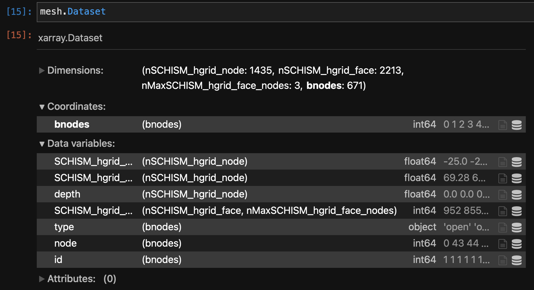
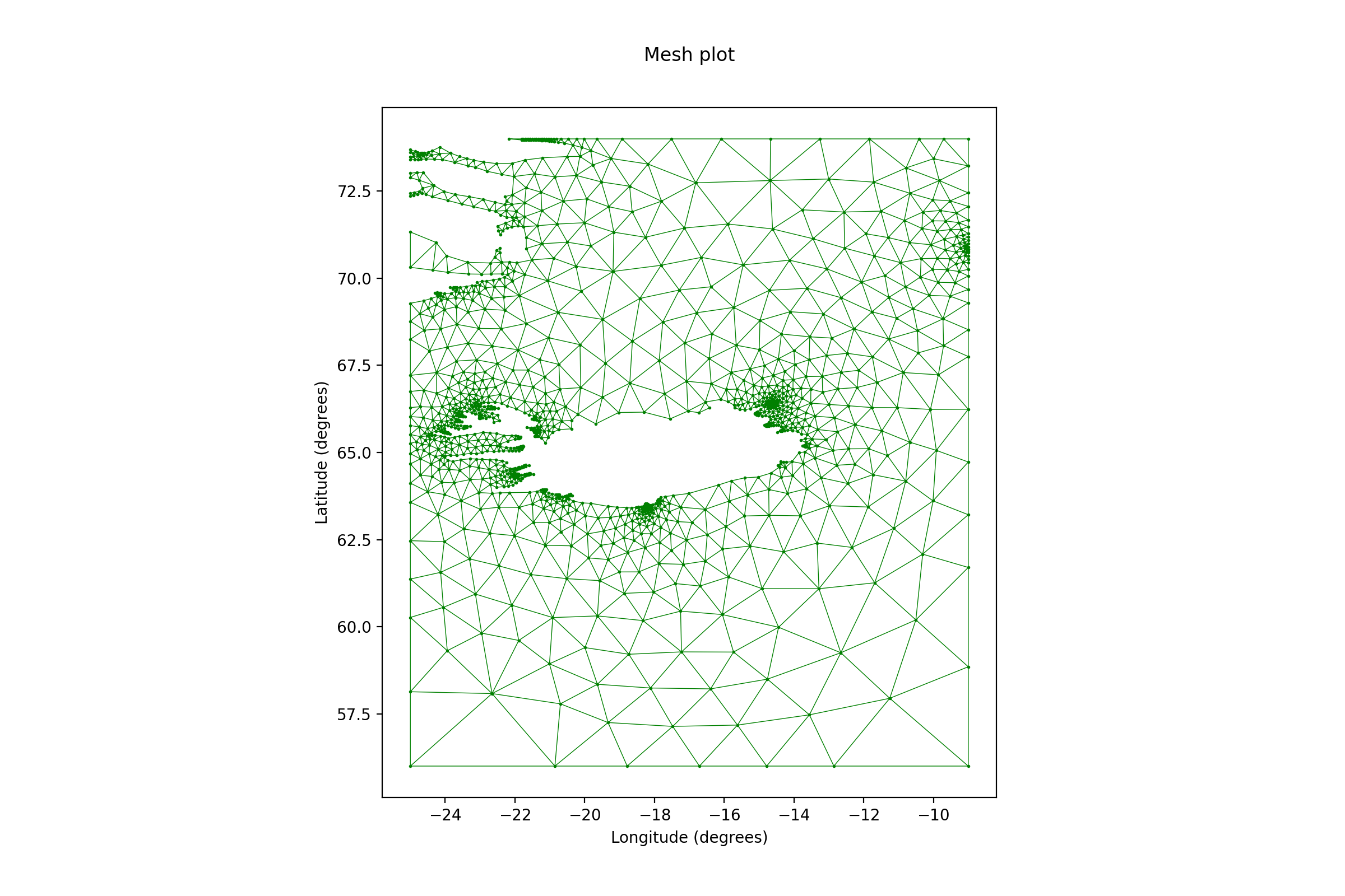
which can be visualised using the inherent accessors (see utils)) with

b.Dataset.pplot.mesh()

Note

You can change the mesh generator above with mesh_generator = gmsh.

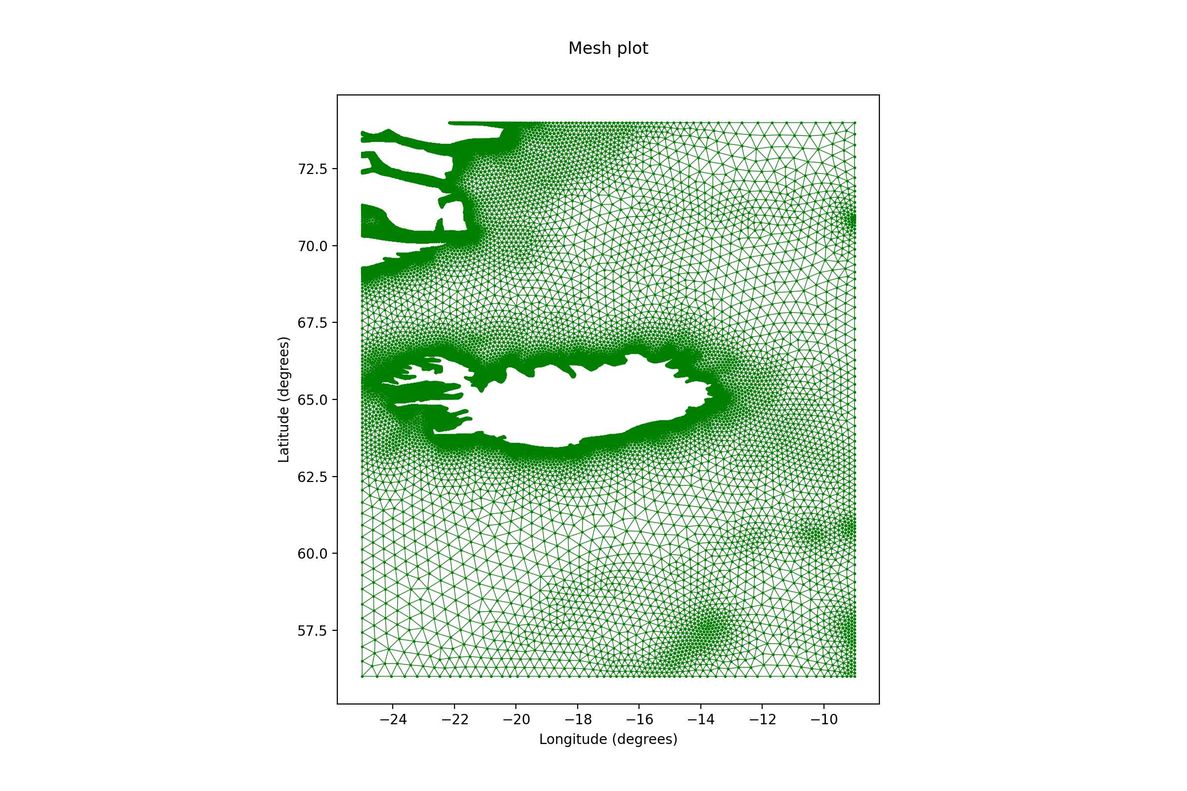
Better control on the mesh size can be obtained by providing a background control function usually in the form of a scaled DEM. One way to achieve this is to give as argument a dem file, like :

b = pm.set(
    type="tri2d",
    geometry=geometry,
    coastlines=iGSHHS,
    mesh_generator="jigsaw",
    dem_source="dem.nc",
    resolution_min=0.01,
    resolution_max=0.5,
)

which gives,

The output to a file, of type hgrid in this case, is done as

b.to_file('/path/to/hgrid.gr3')

There is also a validator that checks whether the mesh works with SCHISM.

b.validate(rpath='/path/to/folder/used/')